LECTURE 1: Probability models and axioms
Two Steps
- Describe possible outcomes
- Describe beliefs about likelihood of outcomes
Sample Space
Sample space is the set of all outcomes of the experiment. It can be discrete or continuous, finite or infinite.
Event: subset of sample space
Probability Axioms and Derived Consequences
Axioms:
- Nonnegativity: $P(A)\ge0$
- Normalization: $P(\Omega)=1$
- (Finite) additivity: if $A\cap B=\phi$, then $P(A\cup B)=P(A)+P(B)$
Consequences:
- $P(A)\le 1$
- $P(\phi)=0$
- $P(A)+P(A^{C})=1$
- For mutually disjoint sets $A_1,A_2,\ldots,A_k$,
$P(A_1\cup A_2\cup\ldots\cup A_k)=P(A_1)+P(A_2)+\ldots+P(A_k)$ - $P(s_1,s_2,\ldots,s_k)=P(\lbrace s_1\rbrace)+P(\lbrace s_2\rbrace)+\ldots+P(\lbrace s_k\rbrace)$
- If $A\subset B$, $P(A)\le P(B)$
- $P(A\cup B)=P(A)+P(B)-P(A\cap B)$
- $P(A\cup B)\le P(A)+P(B)$
- $P(A\cup B\cup C)=P(A)+P(B\cap A^{C})+P(C\cap B^{C} \cap A^{C})$
Probability Calculation
Four Steps
- Specify the sample sapce
- Specify a probability law
- Identify an event of interest
- Calculate
Discrete and Finite
- Two rolls of a tetrahedral die. X for the points of the first roll. Y for the points of the second roll. Sample Space:
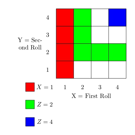
- Discrete uniform probability law: every outcome has the same probability $\frac{1}{16}$.
- $P(X=1)=4\times\frac{1}{16}=\frac{1}{4}$
Let $Z=\min(X,Y)$ - $P(Z=4)=\frac{1}{16}$
- $P(Z=2)=5\times\frac{1}{16}=\frac{5}{16}$
- $P(X=1)=4\times\frac{1}{16}=\frac{1}{4}$
Continuous
- $(x,y)$ such that $0\le x,y\le 1$.
Sample space: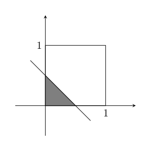
- Uniform probability law: Probability = Area
- $P(\lbrace(x,y)|x+y\le1/2\rbrace)=\frac{1}{2}\times\frac{1}{2}\times\frac{1}{2}=\frac{1}{8}$
Discrete and Infinite
- Tossing a coin, record the number of times until its head faces up.
Sample space: $\lbrace 1,2,\ldots\rbrace$
Probability: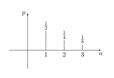
- $P(n)=\frac{1}{2^{n}}$
$P(\text{outcome is even})=P(2)+P(4)+\ldots=\frac{1}{4}\frac{1}{1-\frac{1}{4}}=\frac{1}{3}$
Countable additivity axiom
If $A_1,A_2,\ldots$ is an infinite sequence of disjoint events, then $P(A_1\cup A_2\cup\ldots)=\sum P(A_i)$. It is this axiom that supports the calculation in Discrete and Infinite section. If it is not countable, consider the section Continuous and try to calculate $P(\Omega)$
$$
P(\Omega)=P(\lbrace (x,y)|0\le x,y\le 1\rbrace)=\sum P((x,y))=\sum 0=0.
$$
which is impossible.
Intepretations of probability theory
- (Narrow) a branch of math: Axioms $\Rightarrow$ Theorems
- (Objective) Probability = Frequencies in infinite number of experiments
- (Subjective) Beliefs or Preferences
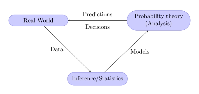
Role of probability theory
- A systematic way of analyzing phenomena with uncertain outcomes
- Whether the probability is useful for making predictions and decisions or not is related to whether the model fits the reality well or not.
- Statistics is to use data from real world to come up with good models for probability theory.
Relation: